The Role of Direct Flights in Trade Costs*

Federal Reserve Bank of Dallas

Globalization and Monetary Policy Institute

Working Paper No. 179

http://www.dallasfed.org/assets/documents/institute/wpapers/2014/0179.pdf

The Role of Direct Flights in Trade Costs

Demet Yilmazkuday

Florida International University

Hakan Yilmazkuday

Florida International University

May 2014

Abstract

The role of direct flights in trade costs is investigated by introducing and using a micro price

data set on 49 goods across 433 international cities covering 114 countries. It is shown that

having at least one direct flight reduces trade costs by about 1,400 miles in distance

equivalent terms, while an international border increases trade costs by about 14,907 miles;

hence, the positive effects of having at least one direct flight between any two cities can

compensate for about 10% of the negative effects of an average international border. Trade

costs also decrease with the number of direct flights: on average, one direct flight reduces

trade costs by about 305 miles in distance equivalent terms, which corresponds to 7% of the

average distance and can compensate for about 2% of the negative effects of an average

international border. The results are shown to be robust to alternative empirical strategies.

JEL codes: F15, F31

Demet Yilmazkuday, Department of Economics, Florida International University, Miami, FL 33199. 305-

348-2316. Demet.yilmazkuda[email protected]

Hakan Yilmazkuday, Department of Economics, Florida

International University, Miami, FL 33199. 305-348-2316. Hakan.yilmazkuday@fiu.edu. The views in this

paper are those of the authors and do not necessarily reflect the views of the Federal Reserve Bank of

Dallas or the Federal Reserve System.

1 Introduction

The increase in air transportation/travel due to the technological development in jet aircraft

engines has led to the improvement of global market integration signi…cantly since World

War II. This improvement has b een partly achieved by the increase in air shipment due to

lower air transportation costs,

and partly due to the face-to-face business meetings that

overcome informational asymmetries in international trade.

Besides the obvious role of

air transportation in the integration of the traded goods markets, air travel of individuals

has also contributed to the integration of non-traded goods markets, such as the housing

market and the service sector.

Therefore, there is no doubt that air transportation/travel

has signi…cantly contributed to welfare-improving globalization through reducing trade costs

between regions/countries.

Within this picture, direct ‡ights have gained more importance, because they provide the

cheapest and fastest air transp ortation/travel. For example, Alderighi and Gaggero (2012)

have found that the elasticity of exports to direct ‡ights is about 10%. Similarly, Micco and

Hummels (2007) shows that by the year of 2000, air shipments were representing a third of the value

of U.S. imports and more than half of U.S. exports with countries outside North America. Similarly, again

in 2000, excluding land neighbors, the air share of import value was more than 30 percent for Argentina,

Brazil, Colombia, Mexico, Paraguay, and Uruguay.

As Cristea (2011) and Poole (2013) have shown, business travel helps to overcome informational asym-

metries in international trade by generating international sales in the form of new export relationships.

For example, Ley and Tutchener (2001) show how house prices in Canadian cities are strongly associated

with overseas tourism. Moreover, service sectors such as medical tourism have bene…ted from the existence

of direct ‡ights b etween countries, as discussed in Bookman and Bookman (2007), Herrick (2007), and Helble

(2011).

Serebrisky (2006) have shown that Open Skies Agreements between countries, which allow

airlines to operate direct ‡ights internationally, reduce air transport costs by 9% and increase

by 7% the share of imports arriving by air. Moreover, studies such as Bel and Fageda (2008)

have found that the availability of direct ‡ights has a large in‡uence on the location of large

…rms’headquarters, which is another factor facilitating trade.

This paper attempts to measure the e¤ects of direct ‡ights on overall trade costs between

cities (in distance equivalent terms) by introducing and using a micro price data set on 49

goods across 433 international cities covering 114 countries. In the benchmark speci…cation,

following Eaton and Kortum (2002), together with other studies in which consumers search

for the minimum price across locations, we de…ne intercity trade costs as the maximum price

di¤erence (i.e., the maximum of deviations from the Law of One Price) across go ods between

two cities; for any city pair for which we compare micro prices, we also search for airports

within 50 miles to check whether they have any direct ‡ights between each other.

The benchmark results show that having at least one direct ‡ight corresponds to a re-

duction in trade costs by ab out 1,400 miles in distance equivalent terms, on average; this is

about one third of the average distance between the cities in the sample that is about 4,551

miles. Due to having both international and intranational city pairs, we also investigate

the role of an international border in trade costs: it is found that the average international

border increases trade costs by about 14,907 miles in distance equivalent terms, which is

about triple the average distance. In other words, the positive e¤ects of having at least one

direct ‡ight between any two cities can compensate for about 10% of the negative e¤ects

Regarding the importance of time spent in transportation, Hummels and Schaur (2013) estimate that

each day in transit is equivalent to an ad-valorem tari¤ of 0.6% to 2.3%.

of an average international border. Trade costs are also shown to be decreasing with the

number of direct ‡ights: the results show that one direct ‡ight reduces trade costs by about

305 miles, which is about 7% of the average distance; therefore, the positive e¤ects of one

direct ‡ight between any two cities can compensate for about 2% of the negative e¤ects of

an average international border.

For robustness, we consider many alternative empirical strategies. In order to measure

trade costs, for instance, we alternatively follow Borraz et al. (2012) who have suggested

using 80th, 90th or higher percentiles of micro price di¤erences in order to reduce the severity

of measurement errors in prices; on the other hand, we also follow Eaton and Kortum (2002)

by using the second maximum of the price di¤erence b etween cities. Since direct ‡ights can

be used for the air transportation of goods (i.e., for the market integration of traded goods)

or for the air travel of individuals (i.e., the market integration of non-traded goods, such

as housing and services, especially through tourism), we also consider the price di¤erence

between cities for both traded and non-traded goods in our sample. Finally, while searching

for a direct ‡ight between any two cities, we consider airports within 25, 100 and 200 miles

of the city centers. In all of these alternative empirical strategies, we …nd very similar results

in which the e¤ect of direct ‡ights on trade costs is always negative and signi…cant.

The rest of the paper is organized as follows. The next section introduces the empirical

methodology used to measure trade costs and details of the regression analysis. Section 3

depicts the data and descriptive statistics. Section 4 reveals the empirical results. Section 5

concludes.

2 Empirical Methodology

2.1 Measuring Trade Costs

Data for trade costs are either non-existing or not covering the globe.

Accordingly, studies

such as by Eaton and Kortum (2002), Simonovska and Waugh (2014), among many others,

have considered disaggregate price information across countries to measure trade costs. For

example, in Eaton and Kortum (2002), given a pair of countries, the maximum price dif-

ference across goods is used as a measure of trade costs. In order to understand the logic

behind this, consider the following arbitrage condition for the same good between any two

locations:

 

(1)

where P

is the price of good g in location i, P

is the price of good g in location j, and 

represents the gross multiplicative trade costs from location j to location i. When traded

goods are considered, this expression literally means that importing good g from location

j is more costly compared to the already-available price in location i; therefore, this is

an expected situation in the equilibrium after arbitrage opportunities are taken (i.e., after

possible trade is achieved). When non-traded goods are considered, this expression means

that travelling from city i to city j to consume good g is more expensive than consuming the

same good in city i; the same arbitrage conditions are implied as for traded goods. Therefore,

An exception is the data set for the U.S. international trade that can be obtained from

http://dataweb.usitc.gov/. Nevertheless, even this detailed data set covers only the calculated duties and

the cost of all freight, insurance, and other charges incurred; it does n ot cover, for instance, trade costs due

to search frictions or time to ship.

in our empirical investigation, b elow, we will consider the implications for both traded and

non-traded goods.

The symmetric version of Equation 1 also holds with an inequality:

 

When trade costs are symmetric (i.e., when 

= 

), the last two inequalities can be

combined in log terms as follows:



 p



 log 

where jj is the absolute operator, p

= log P

, and p

= log P

. The main point is that, when

the maximum (i.e., the upper bound) of the left hand side is considered, the last inequality

turns into an equality. For example, Eaton and Kortum (2002) consider the maximum of the

left hand side as the maximum price di¤erence across goods between two locations, which

can be summarized as follows:

log 

= max





 p





(2)

We follow this de…nition of trade costs in our benchmark results.

As mentioned by Eaton and Kortum (2002) and Borraz et al. (2012), however, the maxi-

mum price di¤erence across goods is sensitive to the possibility of measurement errors in the

price data. Accordingly, Eaton and Kortum (2002) have considered the second maximum

price di¤erence across goods, while Borraz et al. (2012) have considered alternative per-

centiles (e.g., 80th, 90th, etc.). Therefore, besides our benchmark case de…ned as Equation

2, for robustness, we will also consider these alternative measures in our investigation.

2.2 Regression Analysis

Once trade costs are obtained (as described in the previous subsection), we are interested in

the e¤ects of having direct ‡ights between cities. Since we have data for the exact number

of direct ‡ights between cities, we will consider two alternative approaches.

In the …rst speci…cation, we consider the e¤ects of having at least one direct ‡ight between

cities. Accordingly, the following regression will be used (where the superscripts represent

the speci…cation):

log 

= 

+ 

log d

+ c

(3)

where f

is a dummy variable taking a value of 1 when there is at least one direct ‡ight

between cities i and j, b

is a dummy variable taking a value of 1 when there is an interna-

tional border between cities i and j, d

is the great circle distance in miles between cities i

and j, c

and c

are city …xed e¤ects.

In the second speci…cation, we will consider the e¤ects of the number of direct ‡ights be-

tween cities, where we will employ the following regression (where the superscripts represent

the speci…cation):

log 

= 

+ 

log d

+ c

(4)

where f

is the number of direct ‡ights between cities i and j, and the remaining notation

of variables is the same as in the …rst speci…cation, above.

In both speci…cations, the expected sign of 

is negative since we expect that having

direct ‡ights between any considered city pair is going to reduce trade costs due to the

reduced search costs, informational asymmetries, time-to-ship, etc. As consistent with the

literature (e.g., Engel and Rogers, 1996), we also expect the e¤ects of international borders

and distance to be positive (i.e., 

> 0 and 

> 0).

Using the estimated coe¢ cients, following the methodology introduced by Parsley and

Wei (2001), which is robust to the units of distance measurement used (e.g., miles versus

kilometers), the distance equivalent of having direct ‡ights can be measured by the following

expression:

F = d



exp







 1



(5)

while the distance equivalent of the average international border e¤ect can be measured by

the following expression:

B = d



exp







 1



(6)

where d

is the average distance between cities, which is about 4,551 miles. In these expres-

sions, we literally determine the corresponding change in distance units to compansate for

having direct ‡ights or an international border.

3 Data and Descriptive Analysis

Micro price data include observations of 49 goods (22 traded and 27 non-traded) obtained

from 433 cities (covering 114 countries) for the years between 2010 and 2014. The com-

plete lists of goo ds and cities are given in Online Appendix tables, while the coverage of

cities are depicted on the world map in Figure 1, where we have multiple cities from many

countries. The data have been downloaded from http://www.numbeo.com/ which is the

world’s largest database of user contributed data about cities. Users of Numbeo can enter

the micro prices that they observe either at the good level or by using the price collection

sheet provided by the web page. Since the price data are user contributed, Numbeo uses

alternative metho dologies to …lter out noise data. First, the user provided data are checked

for outliers manually.

Second, one quarter of lowest and highest inputs are discarded as

borderline cases. Third, Numbeo uses heuristic technology that discards data which most

likely are incorrect statistically. Using the price data, we calculate log trade costs according

to Equation 2, where, as indicated in Table 1, the number of city pairs is 90,785, and number

of international city pairs are much higher than the number of intranational city pairs.

The data for direct ‡ights have been obtained from Airline Route Mapper for the year of

2013.

The data include information on 63,149 direct ‡ights from around the world where

the name of the airlines and airports are also provided. Considering the provided airport

codes and names, we determined the exact location of the airports (in terms of their latitudes

and longitudes) and the countries in which they are located by using Google Maps.

By using Google Maps, we also calculated the exact location of cities in our price data

(in terms of their latitudes and longitudes). Considering these locations, we calculated the

great circle distance between them in miles to be used in the regression analysis (see Table

1). Furthermore, in order to determine whether there is a direct ‡ight between any two cities

in our price data, we searched for the airports within 50 miles of the city centers by using the

airport location data we have. We found that for some cities, there are no airports within

50 miles, while for some others, there are more than one airp ort; summary statistics are

provided in Table 1 where the number of direct ‡ights is 10,677 (out of 90,785). For a given

city pair for which prices are compared, we calculated the number of direct ‡ights using the

For example, for a particular price in a city, when values contributed are 5, 6, 20, and 4 in a reasonable

time span, the value of 20 is discarded as a noise.

The web page is http://arm.64hosts.com/.

direct ‡ight data that we have by considering all available airports within 50 miles. In the

empirical investigation, we consider two alternative versions of this information: (i) having

at least one direct ‡ight between cities, and (ii) the exact number of direct ‡ights between

cities.

For robustness, we also considered alternative measures of proximity to the airport

(i.e., airp orts within 25, 100, and 200 miles of city centers); in Table 1, to save space, we

only depict the summary statistics for airports within 100 miles of city centers.

When the maximum price di¤erence across goods is used as the measure of trade costs

between cities and airports within 50 miles of city centers are considered to determine direct

‡ights, the corresponding Kernel density estimates are provided in the upper panel of Figure

2, where the city pairs that have a direct ‡ight between each other have fewer trade costs

between each other, independent of considering traded or non-traded goods. The results

remain the same with a di¤erent magnitude when the 80th percentile of price di¤erence

across goods is used as the measure of trade costs between cities, as depicted in the lower

panel of Figure 2. Therefore, direct ‡ights seems to have a reducing e¤ect on trade costs

between cities. Nevertheless, proving this claim requires a formal investigation, of which

results we depict next.

4 Empirical Results

When the maximum price di¤erence across all goods is used as the measure of trade costs

between cities and airports within 50 miles of city centers are considered to determine direct

The exact number of direct ‡ights is de…ned as one ‡ight in any direction between the considered cities.

For example, an airline serving between two cities inbound and outbound is considered as two di¤erent

‡ights.

‡ights, the results in Table 2 are obtained for the estimation of Equation 3. As is evident, all

considered variables are signi…cant at the 1% level, and the adjusted R-bar squared values

are as high as 0.67 when city …xed e¤ects are included. The main point out of these results is

the negative and signi…cant coe¢ cient estimate of the dummy for having at least one direct

‡ight between the considered cities; this result holds for all eight alternative regressions in

Table 2.

We would like to focus on regression version (4) in Table 2, since it includes all the

considered variables in Equation 3. The distance-equivalent e¤ects of having at least one

direct ‡ight, calculated according to Equation 5, are about 1; 400 miles, while the distance-

equivalent e¤ects of borders, calculated according to Equation 6, are about 14; 907 miles.

Therefore, the positive e¤ects of having at least one direct ‡ight between any international

city pair can compensate for the negative e¤ects of a border by about 10%, on average across

all cities in our sample. When distance elasticity of trade is about one, which is the most

commonly estimated coe¢ cient of log distance in gravity studies (e.g., see Disdier and Head,

2008), this result is comparable to the results in Alderighi and Gaggero (2012) who have

found that the elasticity of exports to direct ‡ights is about 10%. Since the average distance

between the cities in our sample is about 4; 551 miles (according to Table 1), we can safely

claim that the e¤ect of borders are about triple the e¤ects of distance, while having at least

In order to compare this number with the existing literature, consider the following studies that have

used alternative data sets and empirical methodologies: Among many others, Engel and Rogers (1996) have

estimated the distance equivalent of the U.S.-Canada border about 75,000 miles; Parsley and Wei (2001)

have estimated the U.S.-Japan border about 43 000 trillion miles; Yilmazkuday (2012) has estimated the

average border across states of the U.S. about 3,344 miles.

one direct ‡ight reduces the e¤ects of distance by one third.

When we replicate the results in Table 2 using price data on traded goods only, we obtain

the results in Table 3, where the signi…cance and signs of all variables remain the same.

When we consider the implied distance-equivalent e¤ects, according regression version (4),

having at least one direct ‡ight corresponds to about 1; 000 miles, while having a border

corresponds to about 25; 870 miles. Hence, having at least one direct ‡ight between any

international city pair reduces the e¤ects of a border by about 4%, on average across all

cities in our sample, when price data on traded goods only are considered.

When Equation 4 is estimated to investigate the e¤ects of the number of direct ‡ights on

trade costs, the results in Table 2 are replaced by the results in Table 4, where the maximum

price di¤erence across all goods is considered as the measure of trade costs, and airports

within 50 miles of city centers are considered to determine direct ‡ights. As is evident,

again, all considered variables have their expected signs and they are signi…cant at the 1%

level. Having one direct ‡ight reduces trade costs by about 305 miles in distance equivalent

terms, on average; hence, an airline serving both an inbound and an outbound ‡ight between

two cities reduces trade costs by about 710 (= 350  2) miles in distance equivalent terms.

The interesting part of this result is that trade costs are reduced further as the number of

direct ‡ights increases. When we replicate the results in Table 4 by using price data on

traded goo ds only, we obtain the results in Table 5, where one direct ‡ight reduces trade

costs by ab out 241 miles in distance equivalent terms, on average.

We considered many alternative estimation strategies for robustness. These include repli-

cating Tables 2-4 by (i) using price data on non-traded goods only, (ii) considering the second

maximum of price di¤erence across goods between cities as the measure of trade costs, (iii)

considering the 80th percentile of price di¤erence across goods between cities as the mea-

sure of trade costs, and (iv) considering airp orts within 100 miles of city centers. All of

these investigations resulted in virtually similar results (i.e., direct ‡ights a¤ect trade costs

negatively and signi…cantly), which can be found in the Online Appendix of this paper.

5 Conclusion

The e¤ects of direct ‡ights on trade costs have been shown to be negative and signi…cant

across cities around the world. Having at least one direct ‡ight corresponds to a reduction

in trade costs by about 1,400 miles in distance equivalent terms, on average, which is about

one third of the average distance between cities. The results also show that one direct ‡ight

reduces trade costs by about 305 miles, which is about 7% of the average distance. Since

the average international b order is shown to increase trade costs by about 14,907 miles, the

positive e¤ects of having at least one direct ‡ight (respectively, having one direct ‡ight)

between any two cities can compensate for about 10% (respectively, 2%) of the negative

e¤ects of an average international border. Therefore, the results, which are supported by

many alternative robustness analyses, are in favor of international policies such as Open

Skies Agreements that facilitate direct ‡ights and thus reduce trade costs.

The results, for sure, depend on the focus of this paper, which is about the e¤ects of direct

‡ights; alternatively, indirect ‡ights may also be contributing to the reduction of trade costs.

However, indirect ‡ights are hard to measure/capture due to the many alternative routes

Many other alternative measu res can also be investigated by u sing the to-be-published Matlab codes of

this paper.

that one can have; e.g., from New York City, USA to Istanbul, Turkey, there are many

alternative airline routes that one can use regarding indirect ‡ights. Such indirect e¤ects,

nevertheless, can be investigated by considering the network e¤ects of direct ‡ights across

cities, although it is out of the scope of this paper.

References

[1] Alderighi, M. and Gaggero, A. (2012) "Do non-stop ‡ights boost exports?," mimeo.

[2] Bel, G. and Fageda, X., (2008), "Getting there fast: globalization, intercontinental

‡ights and location of headquarters," Journal of Economic Geography, 8(4): 471-495.

[3] Borraz, F., Cavallo, A., Rigobon, R. and Zipitría, L., (2012) "Distance and Political

Boundaries: Estimating Border E¤ects under Inequality Constraints," mimeo.

[4] Cristea, A.D. (2011) "Buyer-seller relationships in international trade: Evidence from

U.S. States’exports and business-class travel," Journal of International Economics, 84:

207–220.

[5] Disdier, A.C. and Head, K. (2008) "The puzzling persistence of the distance exoect on

bilateral trade," The Review of Economics and Statistics 90(1): 37–41.

[6] Eaton, J. and Kortum, S. (2002) "“Technology, Geography, and Trade,”Econometrica,

70(5), 1741–1779.

[7] Engel, C., Rogers, J, (1996), "How wide is the border?" American Economic Review,

86: 1112–1125.

[8] Helble, M. (2011) "The movement of patients across borders: Challenges and opportu-

nities for public health," Bulletin of the World Health Organization, 89: 68–72.

[9] Herrick, D.M. (2007), "Medical Tourism: Global Competition in Health Care," National

Center for Policy Analysis, Policy Report No. 304.

[10] Hummels, D., (2007) "Transportation Costs and International Trade in the Second Era

of Globalization," Journal of Economic Perspectives, 21(3): 131-154.

[11] Hummels, D.L. and Schaur, G., (2013) "Time as a Trade Barrier," American Economic

Review, 103(7): 2935-2959.

[12] Ley, D. and Tutchener, J. (2001) “Immigration, Globalisation and House Prices in

Canada’s Gateway Cities,”Housing Studies, 16: 199-223.

[13] Micco, A. and Serebrisky, T. (2006). "Competition Regimes and Air Transport Costs:

The e¤ects of open skies agreements," Journal of International Economics, 70: 25–51.

[14] Parsley, D.C.,Wei, S.-J., (2001), "Explaining the border e¤ect: the role of exchange rate

variability, shipping costs, and geography," Journal of International Economics, 55(1):

87–105.

[15] Poole,J.P. (2013) "Business Travel as an Input to International Trade," mimeo.

[16] Simonovska, I. and Waugh, M.E., (2014) "The elasticity of trade: Estimates and evi-

dence," Journal of International Economics, 92(1): 34-50.

[17] Yilmazkuday,H. (2012), "How wide is the border across U.S. states?" Letters in Spatial

and Resource Sciences, 5:25–31.

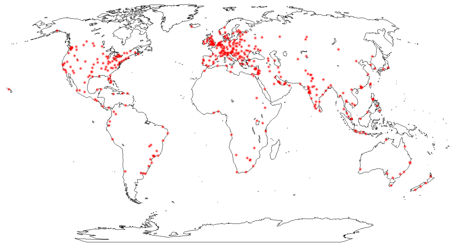
Figure 1 - Cities in the Micro Price Data

Notes: Each star represents a city in the micro price data. There are 433 cities in the sample.

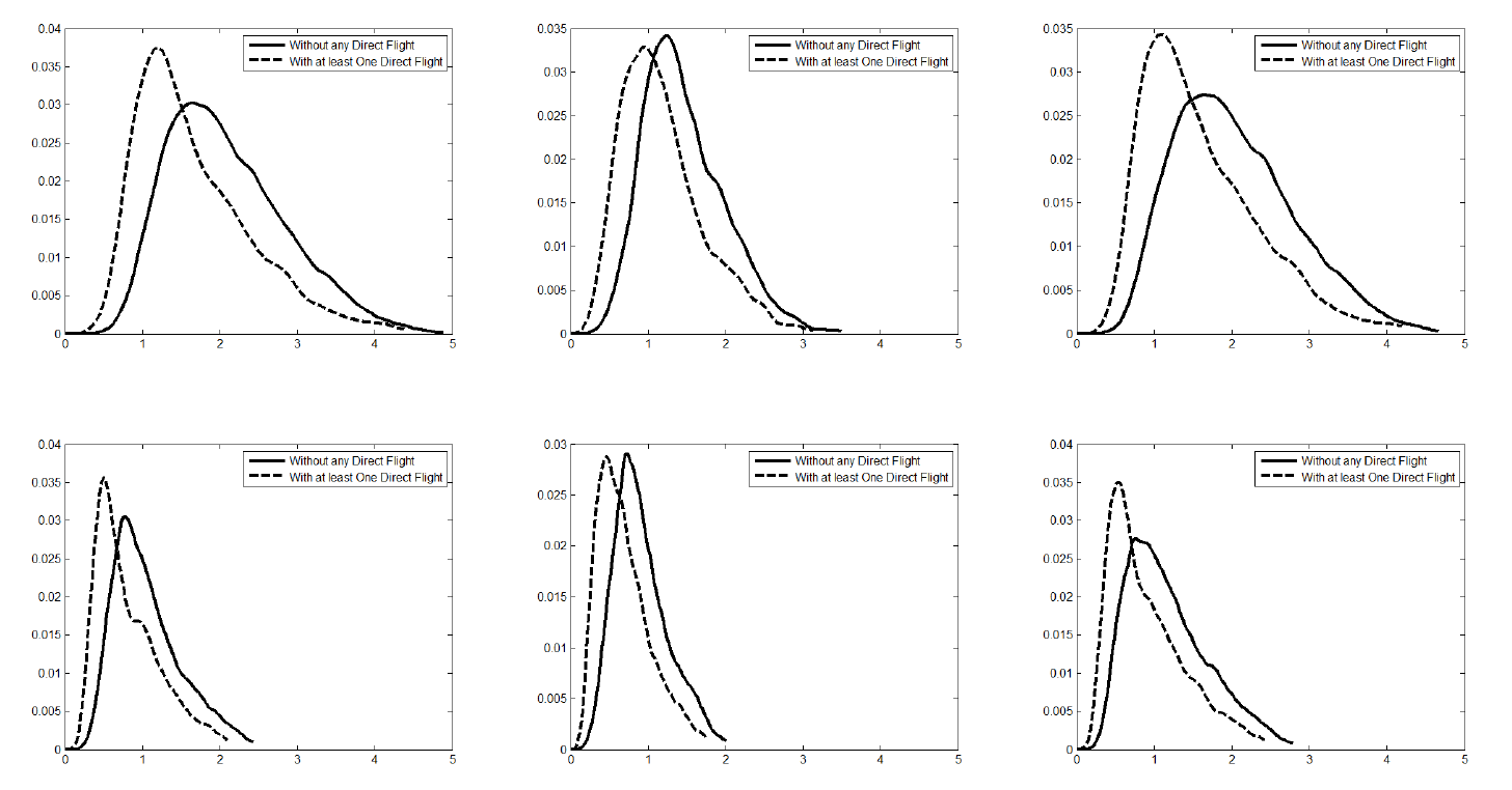
Figure 2 - Kernel Density of Price Dispersion across Cities

Maximum Price Difference across All Goods

Maximum Price Difference across Traded Goods

Maximum Price Difference across Non-Traded Goods

80th Prctile of Price Difference across All Goods

80th Prctile Price of Difference across Traded Goods

80th Prctile of Price Difference across Non-Traded Goods

Notes: For any given city pair and each good, the price difference is first calculated as the absolute log price difference. Afterwards, for each city pair, the

maximum or the 80th percentile of these price differences are calculated across goods. City pairs with direct flights are defined as the pairs that have at least one

direct flight between each other through an airport within 50 miles of the center city. The sample size is 90,785.

Table 1 - Descriptive Statistics

All City Pairs International City Pairs Intranational City Pairs

Number of City Pairs in Price Data 90,785 87,346 3,439

City Pairs that have at least One Direct Flight

through an Airport within 50 Miles

10,677 8,819 1,858

City Pairs that have at least One Direct Flight

through an Airport within 100 Miles

17,135 14,703 2,432

Average Distance in Miles 4,551 4,692 980

Source: International city pairs are defined as the pairs that have an international border between them. Intranational city pairs are defined as the pairs that are

located in the same country. The availability of the price data has been determined by considering the long-run relative prices between 2010-2014. The availability

of the direct flights has been determined according to the data for 2013.

Table 2 - Effects of Having at Least One Direct Flight on the Maximum Price Difference (across All Goods) through an Airport within 50 Miles

Variables Dependent Variable: Maximum (across All Goods) of Absolute Log Price Difference between Cities

(1) (2) (3) (4) (5) (6) (7) (8)

Dummy for Having at Least

One Direct Flight

-0.37***

-0.09***

-0.08***

-0.43***

-0.18***

-0.14***

(0.01)

[0.00]

Log Distance

0.24***

0.21***

0.20***

0.22***

0.21***

0.19***

(0.00)

[0.00]

Border Dummy

0.31***

0.30***

0.51***

0.47***

(0.01)

(0.02)

[0.00]

Distance-Equivalent Effects

of Having at Least One Direct

Flight in Miles

-1,498 -1,400 -2,561 -2,385

Distance-Equivalent Effects

of Borders in Miles

14,817 14,907 49,206 51,555

City Fixed Effects YES YES YES YES NO NO NO NO

R-Squared 0.63 0.67 0.67 0.67 0.02 0.06 0.07 0.07

Notes: *, **, and *** represent significance at the 10%, 5%, and 1% levels, respectively. Standard errors are in parenthesis and p-values are in brackets. All

regressions include a constant that are not shown.

Table 3 - Effects of Having at Least One Direct Flight on the Maximum Price Difference (across Traded Goods) through an Airport within 50 Miles

Variables Dependent Variable: Maximum (across Traded Goods) of Absolute Log Price Difference between Cities

(1) (2) (3) (4) (5) (6) (7) (8)

Dummy for Having at Least

One Direct Flight

-0.29***

-0.06***

-0.04***

-0.29***

-0.13***

-0.09***

(0.00)

(0.01)

[0.00]

Log Distance

0.20***

0.17***

0.16***

0.14***

0.12***

0.11***

(0.00)

[0.00]

Border Dummy

0.32***

0.31***

0.53***

0.51***

(0.01)

(0.02)

[0.00]

Distance-Equivalent Effects

of Having at Least One Direct

Flight in Miles

-1,207 -1,000 -2,743 -2,491

Distance-Equivalent Effects

of Borders in Miles

25,339 25,870 383,948 484,132

City Fixed Effects YES YES YES YES NO NO NO NO

R-Squared 0.64 0.68 0.69 0.69 0.02 0.05 0.07 0.07

Notes: *, **, and *** represent significance at the 10%, 5%, and 1% levels, respectively. Standard errors are in parenthesis and p-values are in brackets. All

regressions include a constant that are not shown.

Table 4 - Effects of the Number of Direct Flights on the Maximum Price Difference (across All Goods) through an Airport within 50 Miles

Variables Dependent Variable: Maximum (across All Goods) of Absolute Log Price Difference between Cities

(1) (2) (3) (4) (5) (6) (7) (8)

Number of Direct Flights

-0.04***

-0.02***

-0.01***

-0.05***

-0.02***

(0.00)

(0.00

(0.00)

[0.00]

Log Distance

0.23***

0.21***

0.20***

0.22***

0.21***

0.19***

(0.00)

[0.00]

Border Dummy

0.31***

0.29***

0.51***

0.46***

(0.01)

(0.02)

[0.00]

Distance-Equivalent Effects

of One Direct Flight in Miles

-305 -305 -476 -434

Distance-Equivalent Effects

of Borders in Miles

14,817 14,479 49,206 46,791

City Fixed Effects YES YES YES YES NO NO NO NO

R-Squared 0.63 0.67 0.67 0.67 0.02 0.07 0.07 0.07

Notes: *, **, and *** represent significance at the 10%, 5%, and 1% levels, respectively. Standard errors are in parenthesis and p-values are in brackets. All

regressions include a constant that are not shown.

Table 5 - Effects of the Number of Direct Flights on the Maximum Price Difference (across Traded Goods) through an Airport within 50 Miles

Variables Dependent Variable: Maximum (across Traded Goods) of Absolute Log Price Difference between Cities

(1) (2) (3) (4) (5) (6) (7) (8)

Number of Direct Flights

-0.03***

-0.01***

-0.03***

-0.02***

-0.01***

(0.00)

(0.00

(0.00)

[0.00]

Log Distance

0.19***

0.17***

0.16***

0.14***

0.12***

0.11***

(0.00)

[0.00]

Border Dummy

0.32***

0.30***

0.53***

0.50***

(0.01)

[0.00]

Distance-Equivalent Effects

of One Direct Flight in Miles

-252 -241 -561 -507

Distance-Equivalent Effects

of Borders in Miles

25,339 25,563 383,948 430,132

City Fixed Effects YES YES YES YES NO NO NO NO

R-Squared 0.64 0.68 0.69 0.69 0.02 0.06 0.07 0.07

Notes: *, **, and *** represent significance at the 10%, 5%, and 1% levels, respectively. Standard errors are in parenthesis and p-values are in brackets. All

regressions include a constant that are not shown.

Online Appendix (Not For Publication)

Table A.1 - Goods in the Micro Price Data

Good Code

Goods

Traded Goods

Meal, Inexpensive Restaurant

Meal for 2, Mid-range Restaurant, Three-course

Combo Meal at McDonalds or Similar

Domestic Beer (0.5 liter draught)

Imported Beer (0.33 liter bottle)

Coke/Pepsi (0.33 liter bottle)

Water (0.33 liter bottle)

Milk (regular), (1 liter)

Loaf of Fresh White Bread (500g)

Eggs (12)

Local Cheese (1kg)

Water (1.5 liter bottle)

Bottle of Wine (Mid-Range)

Domestic Beer (0.5 liter bottle)

Imported Beer (0.33 liter bottle)

Pack of Cigarettes (Marlboro)

One-way Ticket (Local Transport)

Chicken Breasts (Boneless, Skinless), (1kg)

Monthly Pass (Regular Price)

Gasoline (1 liter)

Volkswagen Golf 1.4 90 KW Trendline (Or Equivalent New Car)

Apartment (1 bedroom) in City Centre

Apartment (1 bedroom) Outside of Centre

Apartment (3 bedrooms) in City Centre

Apartment (3 bedrooms) Outside of Centre

Basic (Electricity, Heating, Water, Garbage) for 85m2 Apartment

1 min. of Prepaid Mobile Tariff Local (No Discounts or Plans)

Internet (6 Mbps, Unlimited Data, Cable/ADSL)

Fitness Club, Monthly Fee for 1 Adult

Tennis Court Rent (1 Hour on Weekend)

Cinema, International Release, 1 Seat

1 Pair of Jeans (Levis 501 Or Similar)

1 Summer Dress in a Chain Store (Zara, H&M, ...)

1 Pair of Nike Shoes

1 Pair of Men Leather Shoes

Price per Square Meter to Buy Apartment in City Centre

Price per Square Meter to Buy Apartment Outside of Centre

Average Monthly Disposable Salary (After Tax)

Mortgage Interest Rate in Percentages (%), Yearly

Taxi Start (Normal Tariff)

Taxi 1km (Normal Tariff)

Taxi 1hour Waiting (Normal Tariff)

Apples (1kg)

Oranges (1kg)

Potato (1kg)

Lettuce (1 head)

Cappuccino (regular)

Rice (white), (1kg)

Tomato (1kg)

Notes: Traded goods take a value of 1 in the last column.

Online Appendix (Not For Publication)

Table A.2 - Cities in the Micro Price Data

City

Aachen, Germany

Bhopal, India

Cologne, Germany

Grenoble, France

Kota Kinabalu, Malaysia

Milton Keynes, United Kingdom

Phnom Penh, Cambodia

Sao Jose dos Campos, Brazil

Tunis, Tunisia

Aalborg, Denmark

Bhubenswar, India

Colombo, Sri Lanka

Groningen, Netherlands

Kowloon, Hong Kong

Milwaukee, WI, United States

Phoenix, AZ, United States

Sao Paulo, Brazil

Turin, Italy

Abbotsford, Canada

Bialystok, Poland

Columbus, OH, United States

Guadalajara, Mexico

Krakow (Cracow), Poland

Minneapolis, MN, United States

Phuket, Thailand

Sarajevo, Bosnia And Herzegovina

Turku, Finland

Aberdeen, United Kingdom

Bilbao, Spain

Copenhagen, Denmark

Guangzhou, China

Kuala Lumpur, Malaysia

Minsk, Belarus

Pittsburgh, PA, United States

Saskatoon, Canada

Ulaanbaatar, Mongolia

Abu Dhabi, United Arab Emirates

Birmingham, United Kingdom

Cork, Ireland

Guatemala City, Guatemala

Kuching, Malaysia

Mississauga, Canada

Plovdiv, Bulgaria

Seattle, WA, United States

Utrecht, Netherlands

Accra, Ghana

Bogota, Colombia

Coventry, United Kingdom

Guildford, United Kingdom

Kuwait City, Kuwait

Monterrey, Mexico

Port Elizabeth, South Africa

Seoul, South Korea

Vadodara, India

Ad Dammam, Saudi Arabia

Boise, ID, United States

Cuenca, Ecuador

Gurgaon, India

Lagos, Nigeria

Montevideo, Uruguay

Portland, OR, United States

Sevilla, Spain

Valencia, Spain

Addis Ababa, Ethiopia

Bologna, Italy

Curitiba, Brazil

Haifa, Israel

Lahore, Pakistan

Montreal, Canada

Porto Alegre, Brazil

Shanghai, China

Vancouver, Canada

Adelaide, Australia

Bordeaux, France

Dallas, TX, United States

Halifax, Canada

Larnaca, Cyprus

Moscow, Russia

Porto, Portugal

Sharjah, United Arab Emirates

Varna, Bulgaria

Ahmedabad, India

Boston, MA, United States

Damascus, Syria

Hamburg, Germany

Las Vegas, NV, United States

Mumbai, India

Poznan, Poland

Shenzhen, China

Venice, Italy

Akron, OH, United States

Brampton, Canada

Dar Es Salaam, Tanzania

Hamilton, Canada

Lausanne, Switzerland

Munich, Germany

Prague, Czech Republic

Shiraz, Iran

Verona, Italy

Albuquerque, NM, United States

Brasilia, Brazil

Darwin, Australia

Hanoi, Vietnam

Leeds, United Kingdom

Muscat, Oman

Pretoria, South Africa

Singapore, Singapore

Vicenza, Italy

Alexandria, Egypt

Brasov, Romania

Davao, Philippines

Harare, Zimbabwe

Leicester, United Kingdom

Nagpur, India

Pristina, Serbia

Skopje, Macedonia

Victoria, Canada

Algiers, Algeria

Bratislava, Slovakia

Delhi, India

Hartford, CT, United States

Leiden, Netherlands

Nairobi, Kenya

Puerto Vallarta, Mexico

Sliema, Malta

Vienna, Austria

Alicante, Spain

Brighton, United Kingdom

Denver, CO, United States

Helsinki, Finland

Lille, France

Nanaimo, BC, Canada

Pune, India

Sofia, Bulgaria

Vilnius, Lithuania

Almaty, Kazakhstan

Brisbane, Australia

Detroit, MI, United States

Ho Chi Minh City, Vietnam

Lima, Peru

Naples, Italy

Punta del Este, Uruguay

Split, Croatia

Visakhapatnam, India

Amman, Jordan

Bristol, United Kingdom

Dhaka, Bangladesh

Hobart, Australia

Limassol, Cyprus

Nashville, TN, United States

Quebec City, Canada

Spokane, WA, United States

Vladivostok, Russia

Amsterdam, Netherlands

Brno, Czech Republic

Dnipropetrovsk, Ukraine

Hong Kong, Hong Kong

Lisbon, Portugal

Nasik, India

Quezon City, Philippines

Stavanger, Norway

Warsaw, Poland

Anchorage, AK, United States

Brussels, Belgium

Doha, Qatar

Honolulu, HI, United States

Liverpool, United Kingdom

Navi Mumbai, India

Quito, Ecuador

Stockholm, Sweden

Washington, DC, United States

Ankara, Turkey

Bucharest, Romania

Donetsk, Ukraine

Houston, TX, United States

Ljubljana, Slovenia

New Orleans, LA, United States

Raleigh, NC, United States

Strasbourg, France

Waterloo, Canada

Antalya, Turkey

Budapest, Hungary

Dresden, Germany

Huntsville, AL, United States

Lodz, Poland

New York, NY, United States

Reading, United Kingdom

Stuttgart, Germany

Wellington, New Zealand

Antwerp, Belgium

Buenos Aires, Argentina

Dubai, United Arab Emirates

Hyderabad, India

London, Canada

Newcastle Upon Tyne, United Kingdom

Recife, Brazil

Surabaya, Indonesia

West Palm Beach, FL, United States

Arhus, Denmark

Buffalo, NY, United States

Dublin, Ireland

Iasi, Romania

London, United Kingdom

Nice, France

Regina, Canada

Surat, India

Wichita, KS, United States

Asheville, NC, United States

Bursa, Turkey

Dunedin, New Zealand

Indianapolis, IN, United States

Los Angeles, CA, United States

Nicosia, Cyprus

Reno, NV, United States

Surrey, Canada

Windhoek, Namibia

Athens, Greece

Busan, South Korea

Durban, South Africa

Indore, India

Louisville, KY, United States

Nis, Serbia

Reykjavik, Iceland

Sydney, Australia

Windsor, Canada

Atlanta, GA, United States

Bydgoszcz, Poland

Dusseldorf, Germany

Irbil, Iraq

Luanda, Angola

Nizhniy Novgorod, Russia

Richmond, VA, United States

Szczecin, Poland

Winnipeg, Canada

Auckland, New Zealand

Cairns, Australia

Edinburgh, United Kingdom

Islamabad, Pakistan

Lublin, Poland

Noida, India

Riga, Latvia

Taichung, Taiwan

Wroclaw, Poland

Austin, TX, United States

Cairo, Egypt

Edmonton, Canada

Istanbul, Turkey

Ludhiana, India

Nottingham, United Kingdom

Rijeka, Croatia

Taipei, Taiwan

Yangon, Myanmar

Baghdad, Iraq

Calgary, Canada

Eindhoven, Netherlands

Izmir, Turkey

Lugano, Switzerland

Novi Sad, Serbia

Rio De Janeiro, Brazil

Tallinn, Estonia

Yekaterinburg, Russia

Bahrain, Bahrain

Cambridge, United Kingdom

Esfahan, Iran

Jacksonville, FL, United States

Luxembourg, Luxembourg

Novosibirsk, Russia

Riyadh, Saudi Arabia

Tampa, FL, United States

Yerevan, Armenia

Baku, Azerbaijan

Campinas, Brazil

Espoo, Finland

Jaipur, India

Lviv, Ukraine

Nuremberg, Germany

Roanoke, VA, United States

Tampere, Finland

Yogyakarta, Indonesia

Bali, Indonesia

Canberra, Australia

Florence, Italy

Jakarta, Indonesia

Lyon, France

Odesa, Ukraine

Rochester, NY, United States

Tartu, Estonia

Zagreb, Croatia

Baltimore, MD, United States

Cancun, Mexico

Florianopolis, Brazil

Jeddah (Jiddah), Saudi Arabia

Macao, Macao

Oklahoma City, OK, United States

Rome, Italy

Tashkent, Uzbekistan

Zurich, Switzerland

Bandung, Indonesia

Cape Town, South Africa

Fort Lauderdale, FL, United States

Jerusalem, Israel

Madison, WI, United States

Omaha, NE, United States

Rostov-na-donu, Russia

Tbilisi, Georgia

Bangalore, India

Caracas, Venezuela

Fort Worth, TX, United States

Johannesburg, South Africa

Madrid, Spain

Orlando, FL, United States

Rotterdam, Netherlands

Tehran, Iran

Bangkok, Thailand

Cardiff, United Kingdom

Fortaleza, Brazil

Johor Baharu, Malaysia

Makati, Philippines

Osaka, Japan

Sacramento, CA, United States

Tel Aviv-Yafo, Israel

Banja Luka, Bosnia And Herzegovina

Casablanca, Morocco

Frankfurt, Germany

Kampala, Uganda

Malaga, Spain

Osijek, Croatia

Saint Louis, MO, United States

Thane, India

Barcelona, Spain

Cebu, Philippines

Fredericton, Canada

Kansas City, MO, United States

Malmo, Sweden

Oslo, Norway

Saint Petersburg, Russia

The Hague, Netherlands

Barrie, Canada

Chandigarh, India

Gaborone, Botswana

Karachi, Pakistan

Manama, Bahrain

Ottawa, Canada

Salt Lake City, UT, United States

Thessaloniki, Greece

Basel, Switzerland

Charlotte, NC, United States

Galway, Ireland

Kathmandu, Nepal

Manchester, United Kingdom

Oxford, United Kingdom

Salvador, Brazil

Thiruvananthapuram, India

Beersheba, Israel

Chennai, India

Gdansk, Poland

Katowice, Poland

Manila, Philippines

Padova, Italy

San Antonio, TX, United States

Timisoara, Romania

Beijing, China

Chiang Mai, Thailand

Geneva, Switzerland

Kaunas, Lithuania

Maribor, Slovenia

Panama City, Panama

San Diego, CA, United States

Tirana, Albania

Beirut, Lebanon

Chicago, IL, United States

Genoa, Italy

Kelowna, Canada

Marseille, France

Paphos, Cyprus

San Francisco, CA, United States

Tokyo, Japan

Belfast, United Kingdom

Chisinau, Moldova

Gent, Belgium

Kharkiv, Ukraine

Medellin, Colombia

Paris, France

San Jose, CA, United States

Tomsk, Russia

Belgrade, Serbia

Christchurch, New Zealand

Glasgow, United Kingdom

Khartoum, Sudan

Melbourne, Australia

Patras, Greece

San Jose, Costa Rica

Toronto, Canada

Belo Horizonte, Brazil

Cincinnati, OH, United States

Goa, India

Kiev, Ukraine

Memphis, TN, United States

Pattaya, Thailand

San Juan, Puerto Rico

Toulouse, France

Bergamo, Italy

Cleveland, OH, United States

Goiania, Brazil

Kingston, Jamaica

Merida, Mexico

Penang, Malaysia

San Salvador, El Salvador

Trieste, Italy

Bergen, Norway

Cluj-napoca, Romania

Gold Coast, Australia

Kitchener, Canada

Mexico City, Mexico

Perth, Australia

Santa Barbara, CA, United States

Tripoli, Libya

Berlin, Germany

Coimbatore, India

Gothenburg, Sweden

Kochi, India

Miami, FL, United States

Petaling Jaya, Malaysia

Santiago, Chile

Trondheim, Norway

Bern, Switzerland

Coimbra, Portugal

Graz, Austria

Kolkata, India

Milan, Italy

Philadelphia, PA, United States

Santo Domingo, Dominican Republic

Tucson, AZ, United States

Online Appendix (Not For Publication)

Table A.3-Effects of Having at Least One Direct Flight on the Maximum Price Difference (across NonTraded Goods) through an Airport within 50 Miles

Variables Dependent Variable: Maximum (across Non-Traded Goods) of Absolute Log Price Difference between Cities

(1) (2) (3) (4) (5) (6) (7) (8)

Dummy for Having at Least

One Direct Flight

-0.37***

-0.09***

-0.07***

-0.43***

-0.16***

-0.13***

(0.01)

[0.00]

Log Distance

0.24***

0.21***

0.20***

0.23***

0.22***

0.21***

(0.00)

[0.00]

Border Dummy

0.31***

0.30***

0.46***

0.43***

(0.01)

(0.02)

[0.00]

Distance-Equivalent Effects

of Having at Least One Direct

Flight in Miles

-1,404 -1,286 -2,280 -2,076

Distance-Equivalent Effects

of Borders in Miles

15,112 15,208 30,968 31,164

City Fixed Effects

YES YES YES YES NO NO NO NO

R-Squared 0.57 0.61 0.61 0.61 0.02 0.08 0.08 0.09

Notes: *, **, and *** represent significance at the 10%, 5%, and 1% levels, respectively. Standard errors are in parenthesis and p-values are in brackets. All

regressions include a constant that are not shown.

Online Appendix (Not For Publication)

Table A.4- Effects of the Number of Direct Flights on the Maximum Price Difference (across NonTraded Goods) through an Airport within 50 Miles

Variables Dependent Variable: Maximum (across Non-Traded Goods) of Absolute Log Price Difference between Cities

(1) (2) (3) (4) (5) (6) (7) (8)

Number of Direct Flights

-0.04***

-0.02***

-0.01***

-0.05***

-0.02***

(0.00)

(0.00

(0.00)

[0.00]

Log Distance

0.23***

0.21***

0.20***

0.23***

0.22***

0.21***

(0.00)

[0.00]

Border Dummy

0.31***

0.29***

0.46***

0.41***

(0.01)

(0.02)

[0.00]

Distance-Equivalent Effects

of One Direct Flight in Miles

-317 -319 -429 -388

Distance-Equivalent Effects

of Borders in Miles

15,112 14,771 30,968 28,660

City Fixed Effects

YES YES YES YES NO NO NO NO

R-Squared 0.57 0.61 0.61 0.61 0.02 0.08 0.08 0.09

Notes: *, **, and *** represent significance at the 10%, 5%, and 1% levels, respectively. Standard errors are in parenthesis and p-values are in brackets. All

regressions include a constant that are not shown.

Online Appendix (Not For Publication)

Table A.5 - Effects of Having at Least One Direct Flight on the Second Maximum Price Difference (across All Goods) through an Airport within 50 Miles

Variables Dependent Variable: Second Maximum (across All Goods) of Absolute Log Price Difference between Cities

(1) (2) (3) (4) (5) (6) (7) (8)

Dummy for Having at Least

One Direct Flight

-0.36***

-0.09***

-0.07***

-0.40***

-0.16***

-0.12***

(0.01)

[0.00]

Log Distance

0.23***

0.20***

0.19***

0.20***

0.19***

0.17***

(0.00)

[0.00]

Border Dummy

0.33***

0.32***

0.51***

0.48***

(0.01)

[0.00]

Distance-Equivalent Effects

of Having at Least One Direct

Flight in Miles

-1,505 -1,395 -2,488 -2,273

Distance-Equivalent Effects

of Borders in Miles

18,672 18,989 63,513 67,651

City Fixed Effects

YES YES YES YES NO NO NO NO

R-Squared 0.56 0.60 0.61 0.61 0.03 0.09 0.10 0.10

Notes: *, **, and *** represent significance at the 10%, 5%, and 1% levels, respectively. Standard errors are in parenthesis and p-values are in brackets. All

regressions include a constant that are not shown.

Online Appendix (Not For Publication)

Table A.6 - Effects of the Number of Direct Flights on the Second Maximum Price Difference (across All Goods) through an Airport within 50 Miles

Variables Dependent Variable: Second Maximum (across All Goods) of Absolute Log Price Difference between Cities

(1) (2) (3) (4) (5) (6) (7) (8)

Number of Direct Flights

-0.04***

-0.02***

-0.01***

-0.05***

-0.02***

(0.00)

(0.00

(0.00)

[0.00]

Log Distance

0.22***

0.20***

0.19***

0.21***

0.19***

0.18***

(0.00)

[0.00]

Border Dummy

0.33***

0.31***

0.51***

0.47***

(0.01)

[0.00]

Distance-Equivalent Effects

of One Direct Flight in Miles

-315 -316 -466 -418

Distance-Equivalent Effects

of Borders in Miles

18,672 18,521 63,513 61,633

City Fixed Effects

YES YES YES YES NO NO NO NO

R-Squared 0.56 0.60 0.61 0.61 0.03 0.09 0.10 0.10

Notes: *, **, and *** represent significance at the 10%, 5%, and 1% levels, respectively. Standard errors are in parenthesis and p-values are in brackets. All

regressions include a constant that are not shown.

Online Appendix (Not For Publication)

Table A.7 - Effects of Having at Least One Direct Flight on the 80th Percentile of Price Difference (across All Goods) through an Airport within 50 Miles

Variables Dependent Variable: 80th Percentile (across All Goods) of Absolute Log Price Difference between Cities

(1) (2) (3) (4) (5) (6) (7) (8)

Dummy for Having at Least

One Direct Flight

-0.25***

-0.04***

-0.07***

-0.25***

-0.10***

-0.06***

(0.00)

[0.00]

Log Distance

0.17***

0.15***

0.14***

0.13***

0.11***

(0.00)

[0.00]

Border Dummy

0.29***

0.43***

0.42***

(0.01)

[0.00]

Distance-Equivalent Effects

of Having at Least One Direct

Flight in Miles

-1,001 -714 -2,387 -2,024

Distance-Equivalent Effects

of Borders in Miles

29,621 30,144 211,128 241,002

City Fixed Effects

YES YES YES YES NO NO NO NO

R-Squared 0.43 0.50 0.51 0.51 0.03 0.09 0.12 0.12

Notes: *, **, and *** represent significance at the 10%, 5%, and 1% levels, respectively. Standard errors are in parenthesis and p-values are in brackets. All

regressions include a constant that are not shown.

Online Appendix (Not For Publication)

Table A.8 - Effects of the Number of Direct Flights on the 80th Percentile of Price Difference (across All Goods) through an Airport within 50 Miles

Variables Dependent Variable: 80th Percentile (across All Goods) of Absolute Log Price Difference between Cities

(1) (2) (3) (4) (5) (6) (7) (8)

Number of Direct Flights

-0.03***

-0.01***

-0.03***

-0.01***

(0.00)

(0.00

(0.00)

[0.00]

Log Distance

0.17***

0.15***

0.14***

0.13***

0.11***

(0.00)

[0.00]

Border Dummy

0.29***

0.28***

0.43***

0.41***

(0.01)

[0.00]

Distance-Equivalent Effects

of One Direct Flight in Miles

-290 -287 -484 -418

Distance-Equivalent Effects

of Borders in Miles

29,621 30,198 211,128 222,461

City Fixed Effects

YES YES YES YES NO NO NO NO

R-Squared 0.43 0.50 0.51 0.51 0.03 0.10 0.12 0.12

Notes: *, **, and *** represent significance at the 10%, 5%, and 1% levels, respectively. Standard errors are in parenthesis and p-values are in brackets. All

regressions include a constant that are not shown.

Online Appendix (Not For Publication)

Table A.9 - Effects of Having at Least One Direct Flight on the Maximum Price Difference (across All Goods) through an Airport within 100 Miles

Variables Dependent Variable: Maximum (across All Goods) of Absolute Log Price Difference between Cities

(1) (2) (3) (4) (5) (6) (7) (8)

Dummy for Having at Least

One Direct Flight

-0.36***

-0.08***

-0.07***

-0.42***

-0.18***

-0.15***

(0.01)

[0.00]

Log Distance

0.23***

0.21***

0.20***

0.21***

0.18***

(0.00)

[0.00]

Border Dummy

0.31***

0.30***

0.51***

0.48***

(0.01)

(0.02)

[0.00]

Distance-Equivalent Effects

of Having at Least One Direct

Flight in Miles

-1,318 -1,258 -2,642 -2,623

Distance-Equivalent Effects

of Borders in Miles

14,817 15,481 49,206 62,572

City Fixed Effects

YES YES YES YES NO NO NO NO

R-Squared 0.64 0.67 0.67 0.67 0.03 0.07 0.07 0.07

Notes: *, **, and *** represent significance at the 10%, 5%, and 1% levels, respectively. Standard errors are in parenthesis and p-values are in brackets. All

regressions include a constant that are not shown.

Online Appendix (Not For Publication)

Table A.10 - Effects of Having at Least One Direct Flight on the Maximum Price Difference (across All Goods) through an Airport within 100 Miles

Variables Dependent Variable: Maximum (across All Goods) of Absolute Log Price Difference between Cities

(1) (2) (3) (4) (5) (6) (7) (8)

Number of Direct Flights

-0.02***

-0.01***

-0.03***

-0.01***

(0.00)

(0.00

(0.00)

[0.00]

Log Distance

0.23***

0.21***

0.20***

0.21***

0.18***

(0.00)

[0.00]

Border Dummy

0.31***

0.28***

0.51***

0.44***

(0.01)

(0.02)

[0.00]

Distance-Equivalent Effects

of One Direct Flight in Miles

-155 -147 -286 -260

Distance-Equivalent Effects

of Borders in Miles

14,817 13,848 49,206 46,425

City Fixed Effects

YES YES YES YES NO NO NO NO

R-Squared 0.64 0.67 0.67 0.67 0.03 0.07 0.07 0.08

Notes: *, **, and *** represent significance at the 10%, 5%, and 1% levels, respectively. Standard errors are in parenthesis and p-values are in brackets. All

regressions include a constant that are not shown.